
Getting Census data from multiple years using tidycensus and purrr
This is a follow-up to an earlier blog post where I walked through how to download Census data from multiple state/county combinations using tidycensus and purrr. In this post, I’ll show how to get Census data from multiple years for the same geographic area. This is useful if you want to compare change over time.1
The approach is similar to the prior post: I use purrr::map_dfr() to loop over a list of years and combine the results of get_acs() into one tibble. In this example, I’ll get the total population and median income for each of the nine counties in the San Francisco Bay Area for 2012 and 2017.
library(tidyverse)
library(tidycensus)
library(sf)
library(ggsflabel)
library(scales)

# define years using purrr::lst to automatically creates a named list
# which will help later when we combine the results in a single tibble
years <- lst(2012, 2017)

# which counties?
my_counties <- c(
  "Alameda",
  "Contra Costa",
  "Marin",
  "Napa",
  "San Francisco",
  "San Mateo",
  "Santa Clara",
  "Solano",
  "Sonoma"
  )

# which census variables?
my_vars <- c(
  total_pop = "B01003_001",
  median_income = "B19013_001"
  )

# loop over list of years and get 1 year acs estimates
bay_area_multi_year <- map_dfr(
  years,
  ~ get_acs(
      geography = "county",
      variables = my_vars,
      state = "CA",
      county = my_counties,
      year = .x,
      survey = "acs1",
      geometry = FALSE
      ),
  .id = "year"  # when combining results, add id var (name of list item)
  ) %>%
  select(-moe) %>%  # shhhh
  arrange(variable, NAME) %>%
  print()
## # A tibble: 36 x 5
##    year  GEOID NAME                             variable      estimate
##    <chr> <chr> <chr>                            <chr>            <dbl>
##  1 2012  06001 Alameda County, California       median_income    70500
##  2 2017  06001 Alameda County, California       median_income    96296
##  3 2012  06013 Contra Costa County, California  median_income    74177
##  4 2017  06013 Contra Costa County, California  median_income    95339
##  5 2012  06041 Marin County, California         median_income    90535
##  6 2017  06041 Marin County, California         median_income   113908
##  7 2012  06055 Napa County, California          median_income    68553
##  8 2017  06055 Napa County, California          median_income    86562
##  9 2012  06075 San Francisco County, California median_income    73012
## 10 2017  06075 San Francisco County, California median_income   110816
## # ... with 26 more rows
To compare years, I’ll reshape the data and then calculate absolute change and percent change from 2012 to 2017. I’ll also adjust the 2012 median income estimate for inflation.
# reshape and calculate percent change in income
bay_area_12_17 <- bay_area_multi_year %>%
  spread(year, estimate, sep = "_") %>%
  mutate(
    year_2012 = if_else(
      variable == "median_income",
      round(year_2012 * 1.068449, 0),  # multiply 2012 by cpi inflation factor
      year_2012
      ),
    change = year_2017 - year_2012,
    pct_change = change / year_2012 * 100
    )

# which counties had the largest percent increase in median income?
bay_area_12_17 %>%
  filter(variable == "median_income") %>%
  arrange(desc(pct_change))
## # A tibble: 9 x 7
##   GEOID NAME                variable   year_2012 year_2017 change pct_change
##   <chr> <chr>               <chr>          <dbl>     <dbl>  <dbl>      <dbl>
## 1 06075 San Francisco Coun… median_in…     78010    110816  32806       42.1
## 2 06081 San Mateo County, … median_in…     87195    116653  29458       33.8
## 3 06001 Alameda County, Ca… median_in…     75326     96296  20970       27.8
## 4 06097 Sonoma County, Cal… median_in…     64044     80409  16365       25.6
## 5 06085 Santa Clara County… median_in…     97683    119035  21352       21.9
## 6 06013 Contra Costa Count… median_in…     79254     95339  16085       20.3
## 7 06055 Napa County, Calif… median_in…     73245     86562  13317       18.2
## 8 06041 Marin County, Cali… median_in…     96732    113908  17176       17.8
## 9 06095 Solano County, Cal… median_in…     66314     77133  10819       16.3
From that table, we see that of the nine counties in the Bay Area, San Francisco County had the largest percent increase in median income between 2012 and 2017. The median income in 2012 was $78,010 and it increased to $110,816 in 2017, a percent change of 42.1%.
That table is all well and good, but what if we want to make a map of the data? One of the great things about tidycensus is that it enables you to easily download geometry along with Census estimates.
As I noted in my previous post on this topic , when working with sf objects, it is not possible to use purrr::map_df() or dplyr::bind_rows(). Instead, I will use map() to return a list of sf objects from get_acs() for each year and then combine them with purrr::reduce() and rbind(). One additional wrinkle is to add the year as a new variable to each object in the list before combining.
# loop over year list and get acs estimates with sf geometry
bay_area_multi_year_list <- map(
  years,
  ~ get_acs(
      geography = "county",
      variables = my_vars,
      state = "CA",
      county = my_counties,
      year = .x,
      survey = "acs1",
      geometry = TRUE,
      cb = TRUE
      ),
  ) %>%
  map2(years, ~ mutate(.x, year = .y))  # add year as id variable

# reshape and calculate percent change in income
bay_area_geo <- reduce(bay_area_multi_year_list, rbind) %>%
  select(-moe) %>%
  spread(year, estimate, sep = "_") %>%
  fill(year_2012) %>%
  mutate(
    year_2012 = if_else(
      variable == "median_income",
      round(year_2012 * 1.068449, 0),  # multiply 2012 by cpi inflation factor
      year_2012
      ),
    change = year_2017 - year_2012,
    pct_change = change / year_2012
    ) %>%
  filter(!is.na(year_2017)) %>%
  print()
## Simple feature collection with 18 features and 7 fields
## geometry type:  MULTIPOLYGON
## dimension:      XY
## bbox:           xmin: -123.5335 ymin: 36.89303 xmax: -121.2082 ymax: 38.86424
## epsg (SRID):    4269
## proj4string:    +proj=longlat +ellps=GRS80 +towgs84=0,0,0,0,0,0,0 +no_defs
## First 10 features:
##    GEOID                             NAME      variable year_2012 year_2017
## 1  06001       Alameda County, California median_income     75326     96296
## 2  06001       Alameda County, California     total_pop   1554720   1663190
## 3  06013  Contra Costa County, California median_income     79254     95339
## 4  06013  Contra Costa County, California     total_pop   1079597   1147439
## 5  06041         Marin County, California median_income     96732    113908
## 6  06041         Marin County, California     total_pop    256069    260955
## 7  06055          Napa County, California median_income     73245     86562
## 8  06055          Napa County, California     total_pop    139045    140973
## 9  06075 San Francisco County, California median_income     78010    110816
## 10 06075 San Francisco County, California     total_pop    825863    884363
##    change pct_change                       geometry
## 1   20970 0.27838993 MULTIPOLYGON (((-122.3423 3...
## 2  108470 0.06976819 MULTIPOLYGON (((-122.3423 3...
## 3   16085 0.20295506 MULTIPOLYGON (((-122.4298 3...
## 4   67842 0.06284012 MULTIPOLYGON (((-122.4298 3...
## 5   17176 0.17756275 MULTIPOLYGON (((-122.4463 3...
## 6    4886 0.01908079 MULTIPOLYGON (((-122.4463 3...
## 7   13317 0.18181446 MULTIPOLYGON (((-122.6464 3...
## 8    1928 0.01386601 MULTIPOLYGON (((-122.6464 3...
## 9   32806 0.42053583 MULTIPOLYGON (((-122.332 37...
## 10  58500 0.07083499 MULTIPOLYGON (((-122.332 37...
So now I’ve got the same data as above with the addition of polygons representing the counties. This makes in a breeze to plot with a variety of mapping packages, including ggplot2. Here, I’ll make a choropleth map of the change in median income from 2012 to 2017 by county.
# make that map
bay_area_geo %>%
  filter(variable == "median_income") %>%
  separate(NAME, into = c("name", NA), sep = " County") %>%  # remove
  ggplot() +
  geom_sf(aes(fill = pct_change)) +
  coord_sf(crs = st_crs(bay_area_geo), datum = NA) +
  geom_sf_label_repel(
    aes(label = name),
    fill = "gray95",
    size = 2.5,
    alpha = 0.9
    ) +
  scale_fill_viridis_c("", labels = percent_format(5)) +
  labs(
    title = "Where has median income increased the most?",
    subtitle = "San Francisco Bay Area, 2012 - 2017"
    ) +
  theme_void()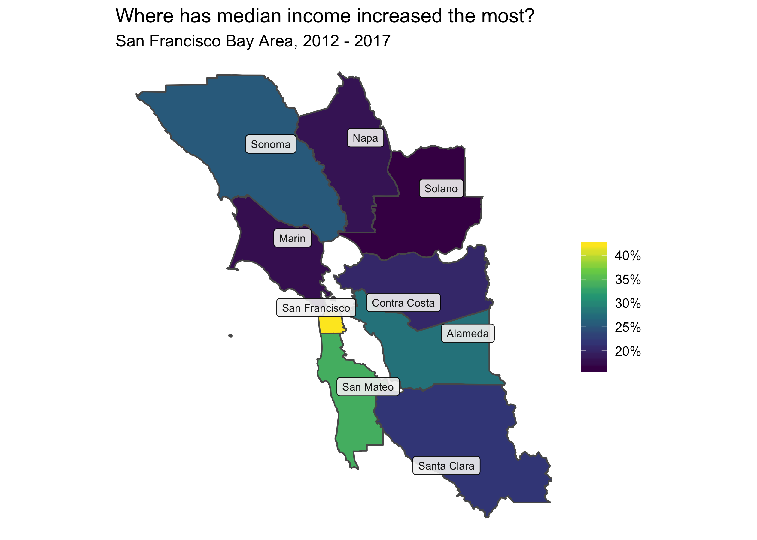
It is important not to use overlapping years when comparing 5-year American Community Survey estimates. For example, you can’t compare 2010-2014 estimates to 2012-2016 estimates, but you could compare 2007-2011 to 2012-2016. In this blog post, I simply use 1-year ACS data which is viable for large geographies (areas with populations greater than 65,000). To compare smaller areas such as census tracts you would need to use non-overlapping 5-year estimates.↩


